Fast Fourier Transformation FFT 快速傅里叶变换 FFT
在音频和声学测量领域,“快速傅里叶变换”(FFT)是一个非常重要的测量方法。它能将一个信号转化为频谱分量,从而得出关于该信号的频率信息。FFT 方法通常适用于对机械或某个系统进行缺陷分析,品质控制以及状态监测等。这篇文章将解释 FFT 如何运作,并介绍相关参数和其对测量结果的影响。
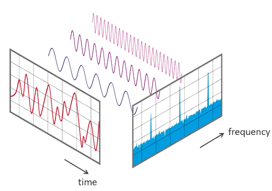
严格来说,FFT 是对“离散傅里叶变换”(DFT)的优化算法实现。信号在一个时间段内被采集并分离出频率分量。这些分量在不同频率各自都是正弦振荡波,有自己的幅度和相位。该转换过程可以用下图来示意。在所测量的时间内,信号包含了三个不同的主频。
信号在时域和频域的视图

Step by step 分步详解
第一步中,信号的一部分被扫描并存储起来用于后处理。这里有两个相关的参数:
- 测试系统的采样率或采样频率 fs(如 48 kHz)。这是一秒内获取的样本平均数量(每秒钟样本数量)
- 选定的样本数量,块长度 BL。在 FFT 中总是 2 的整数幂(如 2^10 = 1024 样本)The sampling rate or sampling frequency fs of the measuring system (e.g. 48 kHz). This is the
从 fs 和 BL 这两个基础参数,可以确定更多的其它参数。
带宽 fn(= 尼奎斯特频率)。这个值表示 FFT 能测得的理论最大频率。
fn = fs / 2
比如采样率为 48 kHz 时,理论上能得到的最大频率分量就是 24 kHz。对于模拟系统来说,由于模拟滤波器的存在,实际测得值通常都或多或少小于理论值,比如说只测到 20 kHz。
测量周期 D。测量周期可由采样率 fs 和块长度 BL 计算。
D = BL / fs.
在 fs = 48 kHz 且 BL = 1024 时,周期即为 1024/48000 Hz = 21.33 ms
频率分辨率 df。频率分辨率表示两个测量结果间的频率间隔。
df = fs / BL
在 fs = 48 kHz 且 BL = 1024 时,分辨率即为 48000 Hz / 1024 = 46.88 Hz
实践中,系统一般都会提供多种可选的采样率。然而,一旦块长度 BL 确定,测量周期和频率分辨率就确定了,可能出现:
- 较小的块长使测量循环更快但频率分辨率较粗
- 较大块长会使测量更慢但得到更好的频率分辨率
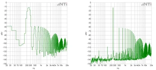 同一信号在较小块长和较大块长下的 FFT 测量结果
以至无限 ...
傅里叶变换中,是假设采集的信号周期性无限重复的,这就带来两个结论:
- FFT 只适用于周期性信号
- 采集的信号段必须包含了一个完整周期
可以看出,结论 2 只有少数信号能满足。如果对一个频率不是 df 的整数倍的信号采样,则在含 2^n 个样本的块内,其将以不同的值开始和结束。这就导致时域信号的跳变,和 FFT 频谱的“弥散”。(也称泄露)
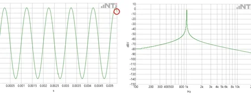
未加时间窗的信号会产生频谱弥散
窗口
为了阻止这种弥散,实践中会对信号样本应用“窗口”。使用一个加权函数,信号样本或多或少会更平缓的开关。这样采集到的和之后的“加窗”信号即以幅值零开始和结束。现在,样本就无需经过复杂的转换而周期性重复。
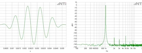
加窗时域信号和频谱
A practical example范例
信号原理中的经典范例就是方波信号的频谱分量。 包含了所有基波频率加权奇数倍之和。

视频以时域信号和频谱形式展现了一个 500 Hz 方波信号是如何产生的。
如何测量?
便携式音频与声学分析仪 XL2 是快速进行简单 FFT 分析的理想工具,最大频率达 20 kHz。对于更多的通道和更详细的分析或计算,就需要像 FLEXUS FX100 音频分析仪这种具备大带宽和快速信号处理器的现代测试系统。与 FX-Control 计算机软件结合,它可以根据测量需要,快速简便的测量和显示 FFT。FX100 的大内存有效支持了更长的块长度,可以得到无比精细的频率分辨率。
FFT 进阶探究
本系列的第二部分将探究对实际的 FFT 测量应用有所帮助的内容。FFT 在众多应用中广泛使用。结果通常为图表因而易于理解。要进行精确的 FFT 测量也有一些细节需要注意。我们将为您提供一些有用的信息。
正如在上篇中所说,测量系统的采样率和块长度 BL 是 FFT 的两个核心参数。采样率表明了扫描待分析信号的速率。比如说,商用级计算机声卡录制 .WAV 格式音频时一般每秒采集 44100 次。
奈奎斯特定理
Harry Nyquist(哈里 · 奈奎斯特)发现了模拟信号采样的一个基础理论:采样率必须至少是信号最高频率的两倍。例如,要对一个最高频率为 24 kHz 的信号采样,采样率就至少要达到 48 kHz。采样率的一半,本例中就是 24 kHz,被称为“奈奎斯特频率”。
如果输入系统的频率高于奈奎斯特频率会怎样呢?
Aliasing 混叠
For the most, a signal is sampled with a more-than-sufficient number of samples. With a 48 kHz sampling rate, for example, the 6 kHz frequency is sampled 8 times per cycle, while the 12 kHz frequency is only sampled 4 times per cycle. At the Nyquist frequency, only 2 samples are available per cycle.
With 2 samples or more it is still possible to reconstruct the signal without loss. If, however, less than 2 samples are available, artifacts which do not occur in the sampled (original) signal are generated.
Mirror frequencies
In the FFT, these artifacts appear as mirror frequencies. If the Nyquist frequency is exceeded, the signal is reflected at this imaginary limit and falls back into the useful frequency band. The following video shows an FFT system with 44.1 kHz sampling rate. A sweep signal of 15 kHz to 25 kHz is fed in to this system.
These unwanted mirror frequencies are counteracted with an analog low-pass filter (anti-aliasing filter) before the scanning. The filter ensures that frequencies above the Nyquist frequency are suppressed.
Time window
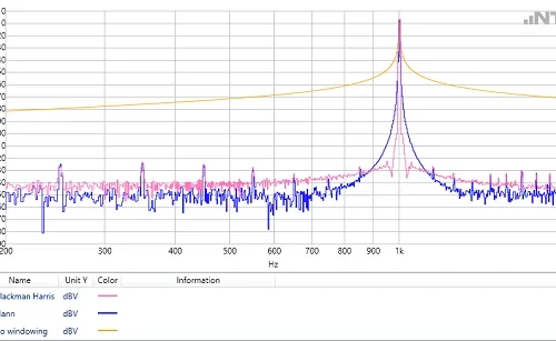
In the case of periodically-continuous signals, the time windowing serves to smooth the undesired transitional jumps at the end of the scanning (see part 1). This prevents smearing in the spectrum. There are numerous types of windows, some of which differ only slightly. When selecting the time window, the following rule applies: Each window requires a compromise between frequency selectivity and amplitude accuracy.
Averaging of Spectra
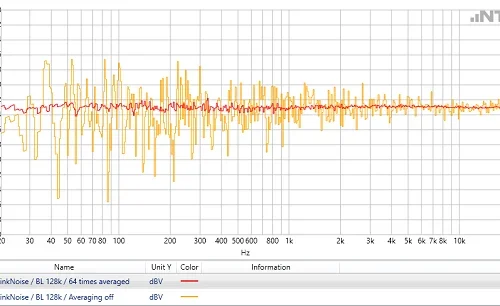
In the analysis of non-periodic signals, e.g. noise or music, it is often advantageous to capture multiple FFT blocks and determine mean values therefrom. There are two possible approaches:
- The classical mean: A number of FFTs are measured. Each result is considered in equal parts in the averaged final result. This method is suitable for measurements with a defined duration.
- The exponential mean: FFTs are continuously measured. Here, too, a fixed number of results of the continuous measurements are considered. However, the weighting is inversely proportional to the ‘age’ of the result. The oldest of the measurements is taken the least into account, the most recent measurement contributes most effectively to the averaged result. This exponential average is used when the spectrum is continuously monitored over a long period of time.
Power vs. Peak detector
Modern high-resolution FFT analyzers offer the possibility to decouple the number of measurement results from the FFT block length. This results in an increase in measurement performance time, especially for high-resolution FFTs. Thus, for example, with a 2MB block length it is no longer necessary to measure and represent more than 1 Million points (bins), but only the number necessary for the display, e.g. 1024.
The value chosen for each FFT bin can be defined in two ways:
- “MaxPeak”: Here the maximum value of the FFT results is used. This type is well suited for the visual representation of FFTs
- “Power”: Here the FFT results are summed up and averaged energetically. This is necessary when the FFT is used for calculations.
Calculations with FFT results
FFTs are mainly used to visualize signals. However, there are also applications where FFT results are used in calculations. For example, very simple levels of defined frequency bands can be calculated by adding them via an RSS (Root Sum Square) algorithm.
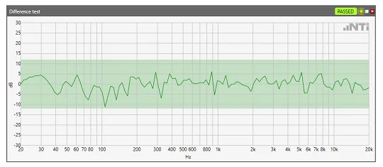
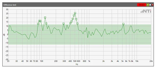
Another application is the comparison of spectra. The example below shows an acoustic measurement of a cordless screwdriver. The measured spectrum is subtracted from a defined reference spectrum. This difference is compared against an upper and lower tolerance. The upper spectrum shows a functional cordless screwdriver. In the lower, the acoustic spectrum suggests that the test specimen is defective.